Queues forming during the Rush Hour

Introduction

This example discusses how it is possible to model the build up of traffic in the rush hour, and thus to see when queues form on a straight road, without junctions, relative to the arrival rate of cars on the section of road.

Symbols Used

Symbol	Represents
Q(t)	Queue length at time t
A(t)	Cumulative arrivals to the queue at time t
D(t)	Cumulative departures from the queue at time t
	The maximum service rate
(t)	The service rate at time t
(t)	Arrival rate at time t

Modelling the Queue

In the rush hour the arrival rate,

(t), will rise until it reaches a maximum rate (i.e. the time when the most people reach the point of road, when they are trying to get to work), after this point the arrival rate will decrease. There are four main points in this flow, as follows:

Time label	Significance
t0	The first point at which (t) equals the maximum service rate,
t1	The point where (t) is a maximum
t2	The point where (t) has decreased back down to
t3	The point where the queue has gone, and so (t) = (t)

The above details tend to imply that a graph of (t) is quadratic, and so would be differentiable twice at or near t1. This means that (t) has a taylor expansion about the point t1:

for constant

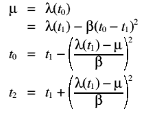
For small t-t1, i.e. this is valid where t0 < t < t3
This means that t0 and t2 can be estimated, by substitution:

Equations for finding t0 and t2

The length of the queue is the area between the curves of (t) and (t), i.e.:

By the using similar substitutions to those used in the previous derivation we can simplify this to:

Henry Morgan, 14 June 1999